Robot-Leg Theory
Taking a cue from quadruped animals, which adjust their stride frequency, reduce contact time, and incorporate lateral swing movements to maintain balance at higher locomotion speeds, I aim to design a leg model that achieves a high-speed gait, minimizes power consumption, and ensures stability.
It's important to note that this text is based on insights from the article "Leg Trajectory Planning for Quadruped Robots with High-Speed Trot Gait," authored by Xuanqi Zeng, Songyuan Zhang, Hongji Zhang, Xu Li, Haitao Zhou, and Yili Fu. I highly recommend delving into the details of their work to further enrich your understanding. The link to the article is provided below for your reference.
Introduction:
The choice of a legged robot over a wheeled or tracked counterpart is straightforward—it proves more adept in navigating rough terrains and complex environments. Given my familiarity with wheeled machines, I acknowledge that delving into legged robots reveals their additional complexity, offering a new challenge and opportunity for innovation. However, there are drawbacks to opting for legs, particularly in terms of power consumption. To simplify the physics involved, consider this analogy:
Imagine a bike and a dog with the same mass moving at identical speeds in the same direction. The bike follows a straight trajectory in the Z-axis, maintaining a constant height. In contrast, the dog's mass center fluctuates as it walks, moving up and down. To illustrate, try holding a chalk at the highest point you can reach, walk, and draw a line—you'll notice it's not a straight line but more of a wavy pattern. This variation in height during walking contributes to increased energy consumption compared to the efficiency of riding a bike.
- The energy used by a bike is given by: \(E_{bike}=E_{k}+ E_{p}= \frac{m v^{2} }{2}+mgh(h=0)\) simplifying to: \(E_{bike}= \frac{m v^{2} }{2} \)
- On the other hand, the energy used by a dog is represented by: \(E_{dog}=E_{k}+ E_{p}= \frac{m v^{2} }{2}+mgh(h>0)\), which further includes potential energy due to height, resulting in: \(E_{dog}= \frac{m v^{2} }{2} +mgh\)
As mentioned earlier, both the car and the dog share the same mass and velocity, yet the energy used by the bike(\(E_{bike} - used\)) is less than that of the dog (\(E_{dog} - used\)): \(E_{bike} used < E_{dog} used\)
Hence, I'll endeavor to optimize energy consumption by selecting suitable actuators and refining the movement path. Other factors such as complexity, cost, and more will also be considered, but I'll delve into those details later.
| Hydraulic actuators | Electric actuators |
| Very difficult design. | Wide cost range. |
| High cost. | Easier design and control system. |
| Large noise and size. | High acceleration. |
| Huge carrying capacity and motion ability. | Lighter. |
| Heavy |
I'll conclude here and proceed by opting for an electric actuator, which aligns better with my DIY projects. It's a cost-effective, lightweight option with sufficient carrying capacity. For a deeper understanding of the differences between electric, hydraulic, and pneumatic linear actuator systems, I highly recommend reading the "Comparative study of a hydraulic, pneumatic, and electric linear actuator system", I've attached the link below. Furthermore, it's worth mentioning in advance that my plan involves designing a simplified 2-joint structure. This approach aims to streamline the project and reduce overall costs.
In the realm of quadruped robots, the application of leg motors generally follows two primary approaches: distributing motors at each joint or consolidating them solely at the shoulder. The first method results in elastic actuation, favorable for dynamic motions. It facilitates steady and controllable walking; however, the drawback lies in the slower swing speed of the legs, leading to a lower overall walking speed. On the other hand, the second option presents a simpler design with minimal mass center changes. It enables the easier design of high-speed movements without concerns about leg inertia. Now, let's delve into the mathematical analysis to craft an optimal leg design.
Kinematic analysis of the leg:
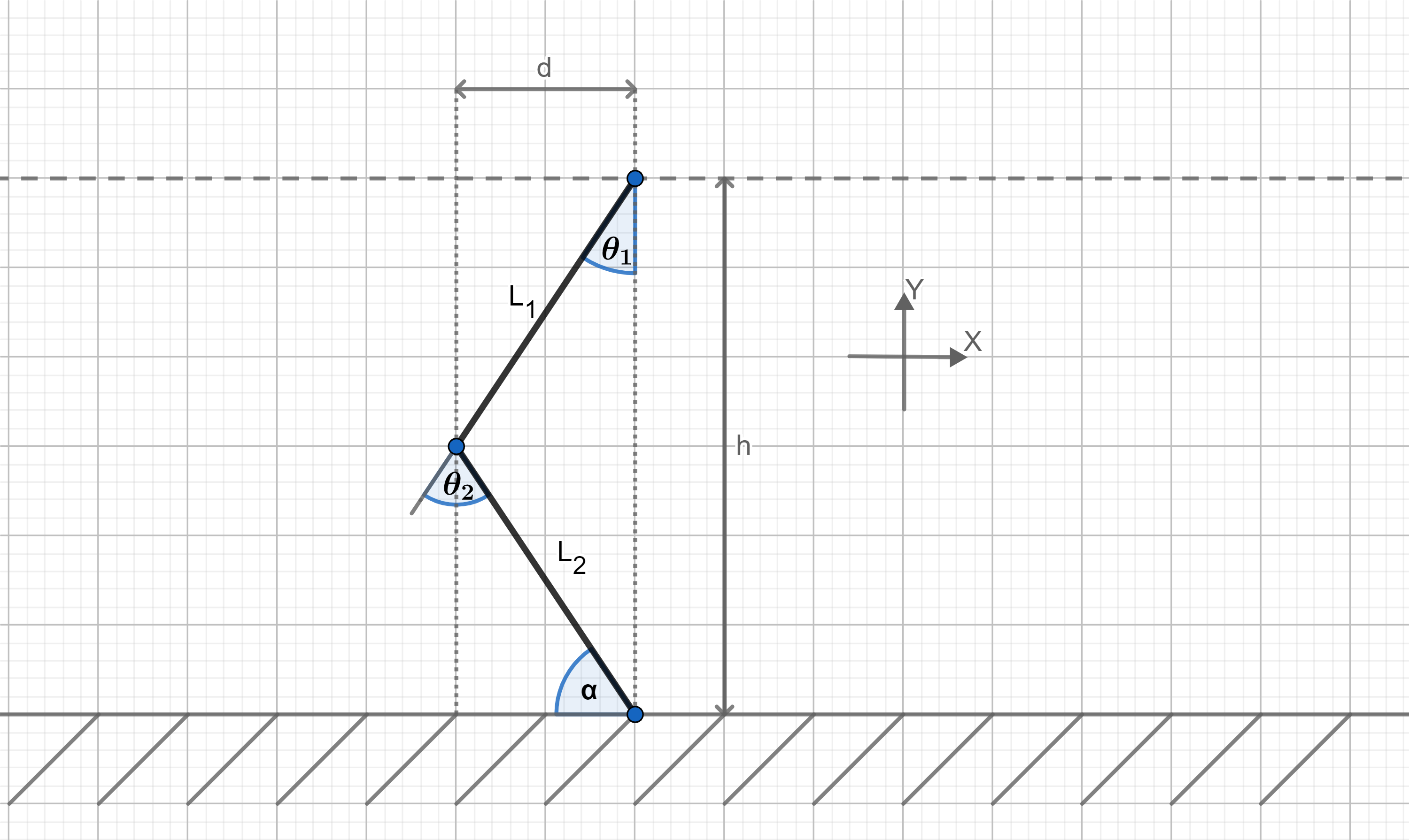
1) Manipulability Measure: In the context of the Manipulability Measure, let's examine a manipulator equipped with 2-degrees of freedom, where the joint variables are represented as \( \Theta _{i} \). When we define the hand position as the manipulation vector \("r"\) with coordinates \([x, y]^{T} \), the corresponding Jacobian matrix is expressed as follows:
\( J( \Theta _{1}, \Theta _{2})=\begin{bmatrix}L_{1}*cos( \Theta _{1})+L_{2}*cos( \Theta _{1}+ \Theta _{2}) & L_{2}*cos( \Theta _{1}+ \Theta _{2}) \\ L_{1}*sin( \Theta _{1})+L_{2}*sin( \Theta _{1}+ \Theta _{2}) & L_{2}*sin( \Theta _{1}+ \Theta _{2}) \end{bmatrix} \)
\(w=|detJ(\Theta_{1}, \Theta_{2})|=L_{1}*L_{2}*sin(\Theta_{2})\)
The consequential factor in this scenario is termed the Jacobian determinant. At a specific point, denoted as \("w"\), it attains its minimum, equivalent to zero. To enhance the manipulability of the leg, a strategic selection of parameters is imperative to maximize the overall output. Hence, the manipulator attains its optimal position when 2 equals ±90 degrees (since \(sin(90^{ \circ } )\), equals 1), and the lengths of \(L_{1}\) and \(L_{1}\) are equal (when \(L_{1}+L_{2}=const\)). To reinforce these findings, consider the daily example of the human arm:
“A two-joint arm (accounting for the shoulder and elbow as 2-degrees of freedom) that approximately adheres to the relationship \(L_{1}=L_{2}\). Moreover, in practical scenarios, when handling objects, the elbow angle tends to hover around the optimum of close to \(90^{ \circ } \), as highlighted in "Manipulability of Robotic Mechanism" by Tsuneo Yoshikawa.”
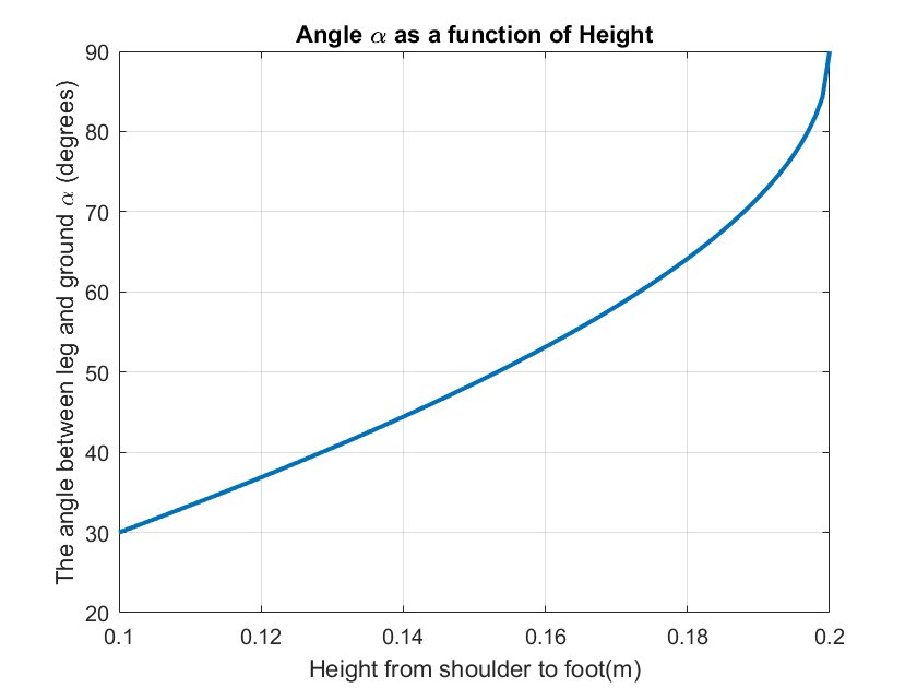
2) Optimum angle \(\alpha \), between the foot and the ground referencing a height from shoulder to foot.
cosine rule: \( L^{2}_{1}= L^{2}_{2}+ h^{2}-2* L^{2}_{2}*h*cos( \beta ) \)
\(\beta\) - is an angle between \(L_{2} \)and \(h\)
\( \alpha = 90^{ \circ } - arcos( \frac{ L^{2}_{2}+ h^{2}- L^{2}_{1} }{2* L_{2}*h } )\)
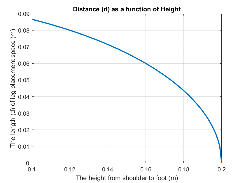
3) The distance between shoulder and knee. Using Heron's Formula.
Half of the triangles perimeter: \(S= \frac{ L_{1}+ L_{2}+h }{2} \)
Heron's formula: \(A= \sqrt{S*(S-L_{1})*(S-L_{2})*(S-h)} \)
Area of triangle: \(A= \frac{h*d}{2} \)
Space occupied: \(d= \frac{2*\sqrt{S*(S-L_{1})*(S-L_{2})*(S-h)} }{h} \)
Inverse Kinematic Analysis:
To determine the optimal paths for our leg, it's crucial to calculate the positions of two joints: the shoulder and the foot. For this task, we employ Inverse Kinematics (IK), which stands in contrast to Direct or Forward Kinematics. In Forward Kinematics, we start from a fixed base (the shoulder) and work our way towards the end effector position (the foot) using Cartesian coordinates. Inverse Kinematics, on the other hand, takes the end effector (foot) as the base, relying on the process of deducing joint angles from known coordinates of the end effector (x and y coordinates of the foot). This enables us to precisely determine the positions of the shoulder and foot joints in our leg model.
(x, y) - is our end effector(foot)
A - is our base point(shoulder)
h - height from shoulder to foot
Pythagoras: \(h^{2}=x^{2}+y^{2}\)
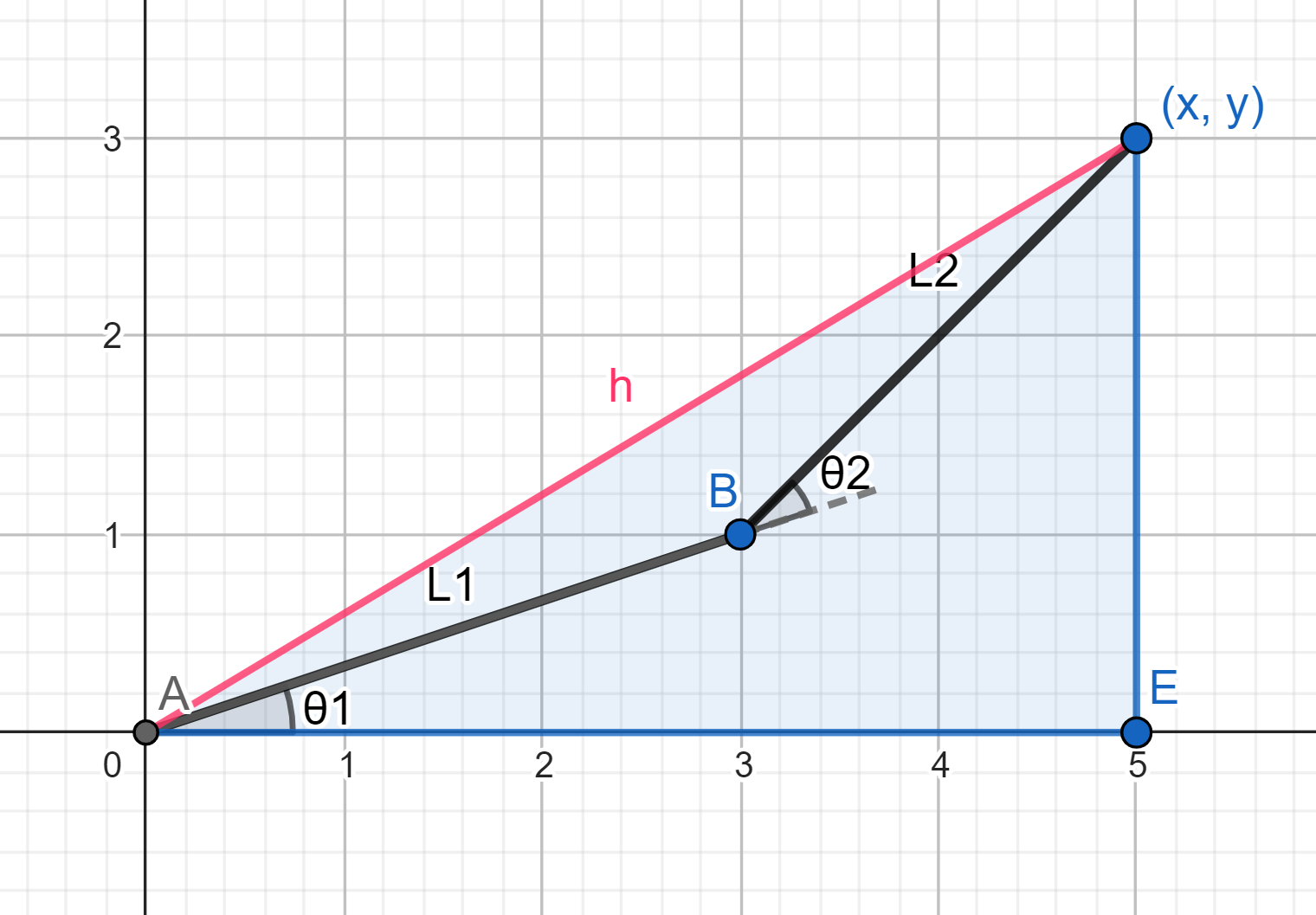
cosine rule: \(h^{2}= L^{2}_{1} *L^{2}_{2}-2*L^{2}_{1} * L^{2}_{2}*cos( \beta ) \)
\(\alpha=180^{ \circ }-\Theta_{2} \), \(h^{2}=x^{2}+y^{2}\)
\(cos(180^{ \circ }-\Theta_{2}) =\frac{ L^{2}_{1}+L^{2}_{2} - x^{2}- y^{2} }{2* L_{1}* L_{2} } \)
\(\Theta_{2}=arcos(\frac{x^{2}+ y^{2} - L^{2}_{1}-L^{2}_{2} }{2* L_{1}* L_{2} } ) \)
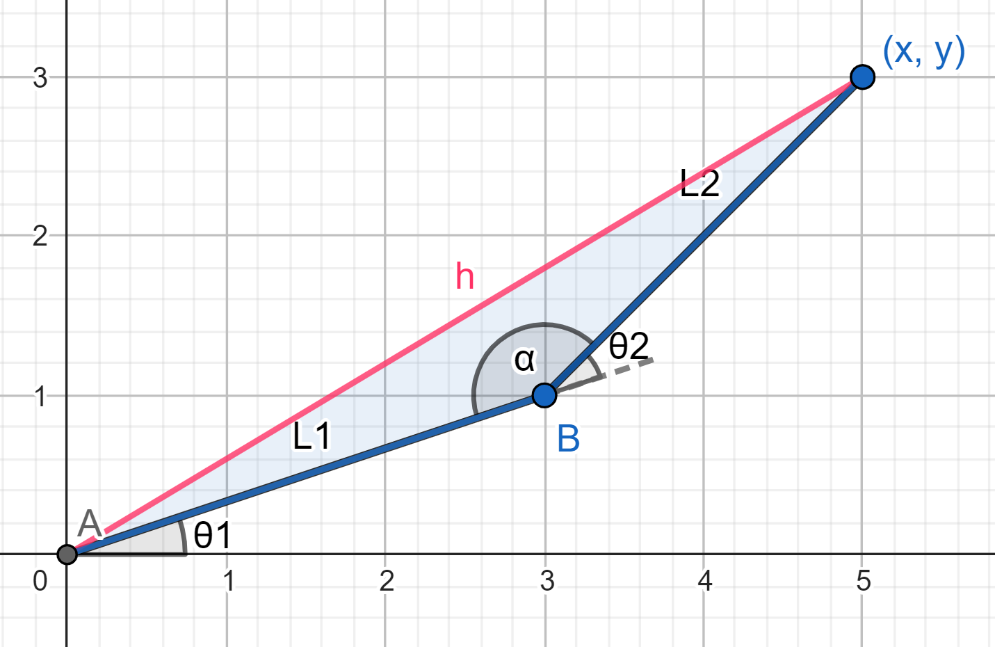
\(\beta \) - angle between h and L1 in point A
\(\beta=arctan( \frac{ L_{2}*sin(\Theta_{2}) }{L_{1}+L_{2}*cos\Theta_{2})} ) \)
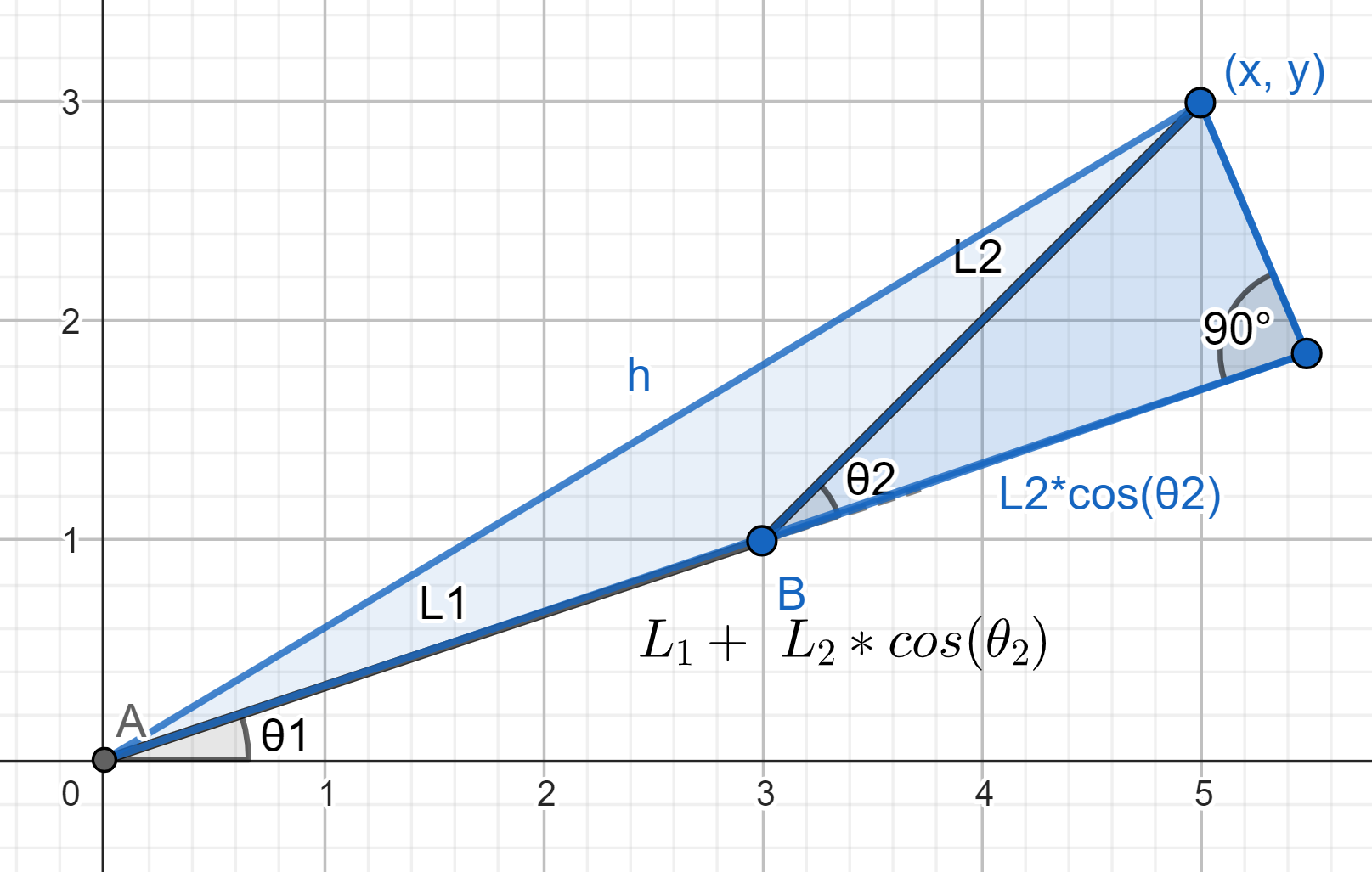
\( \varphi \) - angle between h and X-axis
\( \varphi =arctan( \frac{x}{y} )\)
\(\Theta_{1}= \varphi - \beta \)
\(\Theta_{1}=arctan( \frac{x}{y} )-arctan( \frac{ L_{2}*sin(\Theta_{2}) }{L_{1}+L_{2}*cos\Theta_{2})} ) \)
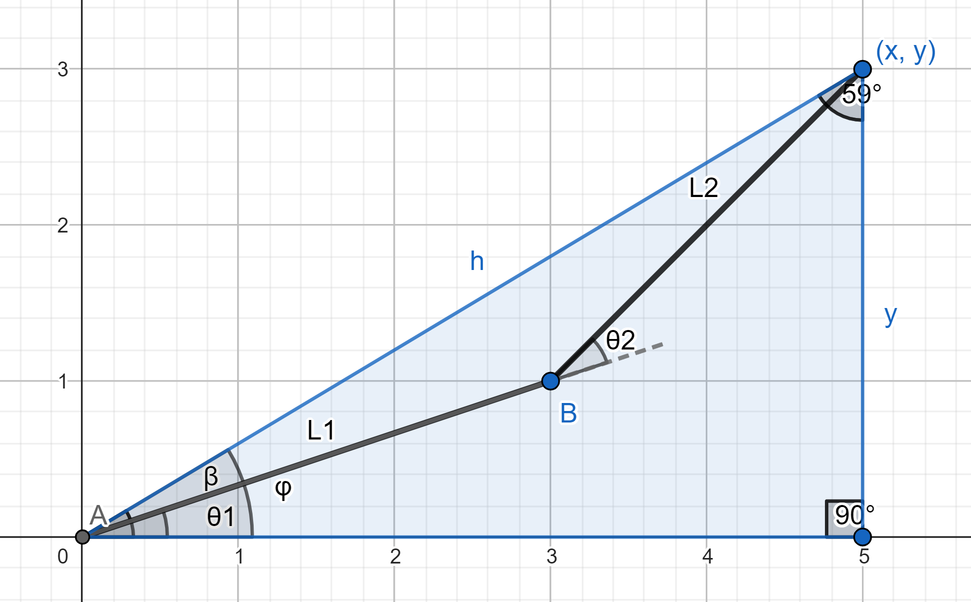
By utilizing these two formulas, we can effortlessly compute the desired position of the foot. In scenarios like a robot arm, such calculations might require additional considerations. For instance, if \(\Theta_{2}\) becomes negative, we might need to adjust the formula by multiplying \(\Theta_{2}\) by \(-1\) and, in \(\Theta_{1}\), change the minus sign to plus. However, in the case of legs, where the knee only bends in one direction, this complexity is eliminated, and we can proceed without such concerns.
In our upcoming installment, we'll venture deeper into the heart of this synergy, illuminating the process of translating these design principles into tangible mechanical structures and intricate 3D models. Furthermore, we'll uncover the hidden secrets behind crafting the code for the seamless motion of robot legs. From conceptualization to realization, we'll unravel the intricacies of bringing these robotic marvels from the drawing board to reality.
Comments
William
- 04 March, 2024
Amazing!
Leave a comment