Robot Dog
Introduction
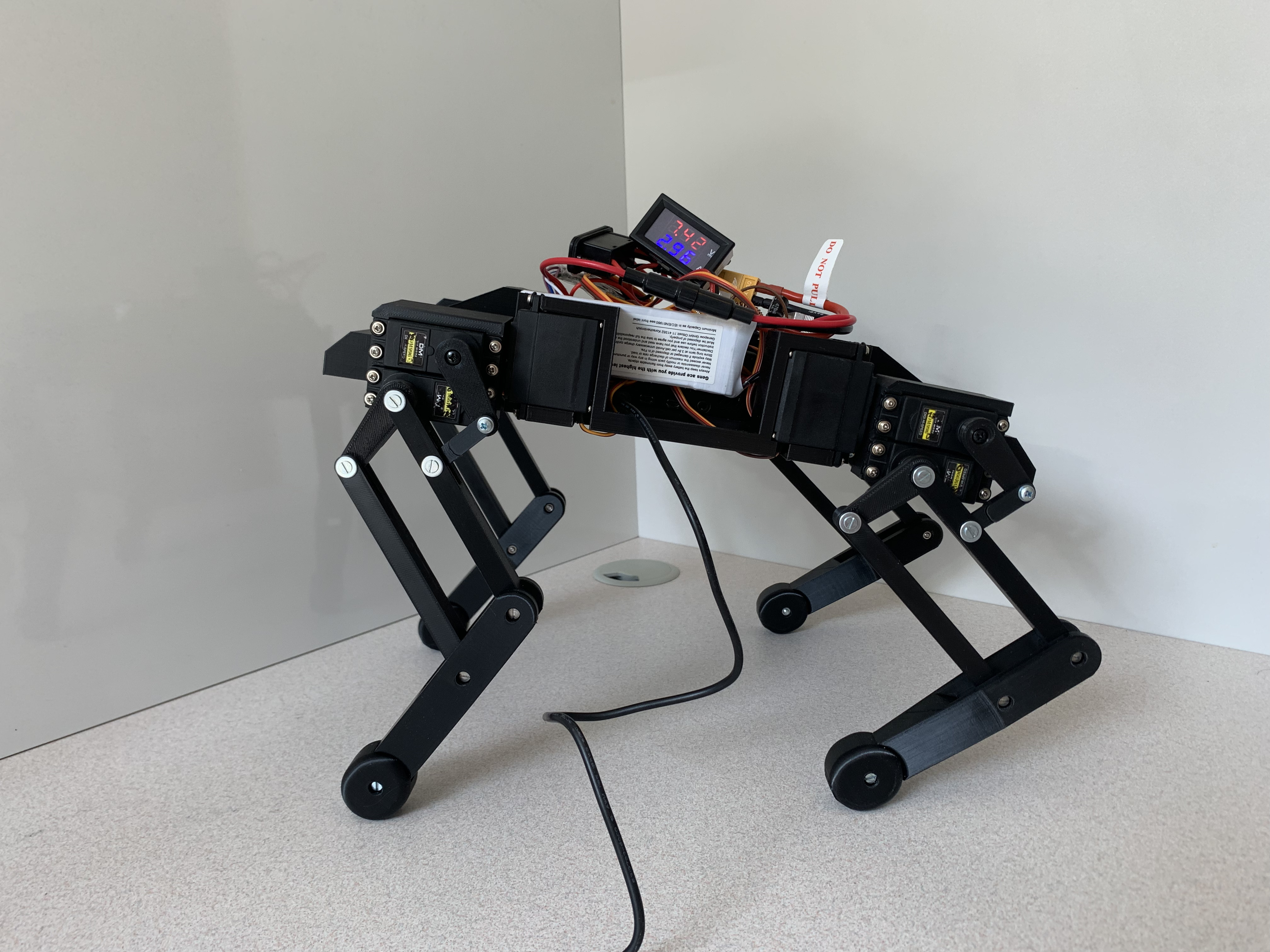
Continuing my journey in creating and implementing a robot dog, the time has come to print the parts and assemble them. This process took over 40 hours of continuous printing. As always, when transitioning from design to reality, there are a few aspects I could improve or change, which I will discuss in this article. While I can't promise this will be the last post on this project or that all my goals will be achieved, we'll see what the future holds.
I also want to mention that I won't delve deeply into topics I've already covered in other articles, such as inverse kinematics, leg design, or leg simulation. Without further ado, enjoy your reading!
External Parts
What You Need:
- 12x Servos
- Buck Converter
- Raspberry Pi 4B
- High-Amperage Switch
- PCA9685 (to control 12 servos)
- Battery 7.4V, 30C (to handle the high amperage draw without damaging the battery)
- Screws:
- 12x M3x12mm
- 4x M3x10mm
- 8x M3x20mm
- 4x M3x14mm
- 8x M3x18mm
- 32 M3 Nuts
- 20 M3 Washers
Additional:
- 20A Fuse (to protect the buck converter)
- Fuse Holder
- Multimeter (Although it can only handle up to 10A, it is sufficient for calibrating the buck converter)
Design and Printing
If you want to print your robot dog, check out my Thingiverse profile. Let's start from the beginning, with the 3D model. My main goal was to create a robot the size of a small dog, with easily replaceable parts and straightforward assembly. This meant using as few screws as possible. In the end, I believe I achieved these three objectives. Overall, assembling the robot requires only 36 screws (not including the screws provided in the servo kit). The leg offers three dimensions of movement with a reliable, rigid body. The robot consists of 21 parts: each leg has 8 parts, and the body is built from 3 parts (with an optional top cover extension). Each leg uses 3 servos. For more details on leg design, I recommend reading my previous post.
For the body, I designed just three parts to simplify assembly: the "Back Bumper," "Front Bumper," and "Body." Assembling these three parts requires only 8 M3x20mm screws.
During printing, you need to mirror four parts for the left and right sides in your slicing program: "Shoulder-Front," "Shoulder-Back," "Thigh-Lower," and "Thigh-Upper." Alternatively, you can download ready-to-use files from my Thingiverse profile. I use Cura for slicing, which I highly recommend.
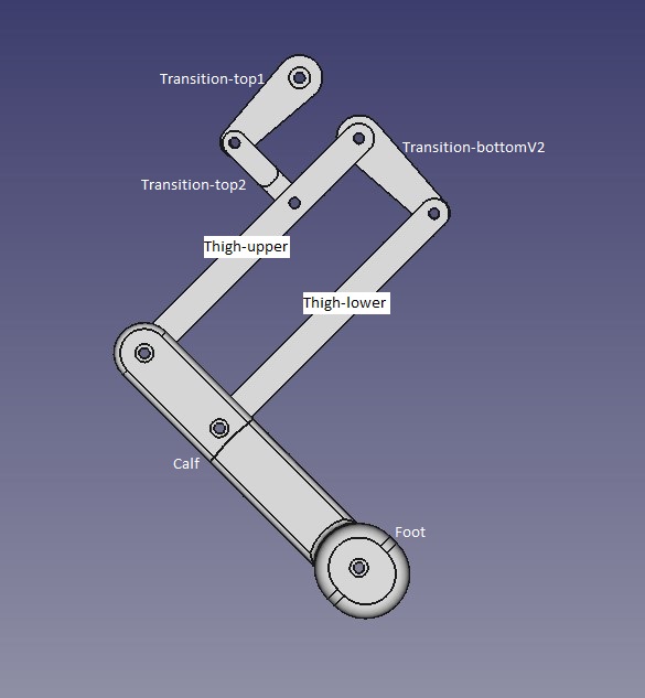
Printing Data (Quality 0.2 mm, Adhesion and Support On, 0.4 Nozzle):
-
100% Infill:
- Transition-top1
- Transition-top2
- Transition-bottomV2
- 20% Infill:
- Thigh-upper Right
- Thigh-lower
- Calf Right
- Foot
- Shoulder
- Body
- Front Bumper
- Back Bumper
Assembling
Before mounting parts to the servos, you need to calibrate all the servos to their starting positions:
- Servo top (S1) - 0 degrees
- Servo bottom (S2) - 0 degrees
- Shoulder servo (S3) - 90 degrees
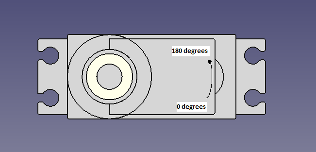
You can easily accomplish this using one of the codes in the Python library (servo_calibration.py). Additionally, I recommend marking the servos to indicate 0 and 180 degrees and their rotation directions. Once calibrated, you can begin assembling them.
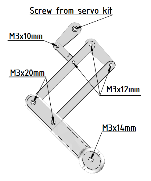
Step-by-Step Assembly:
Assemble the Legs:
You need to assemble four legs, two right and two left, as shown in the picture below.
- Start from the bottom: screw the foot to the calf, then attach the calf to the lower and upper thigh.
- Ensure that the larger holes for the nuts are directed inward. For the right leg, when the leg is directed forward, the larger holes in the upper part should be on the left side (refer to the picture below).
- Attach the transition top2 to complete the leg assembly.
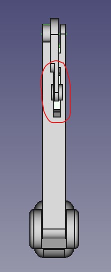
Mounting the Servos:
- Once all four legs are assembled, begin mounting the servos to the shoulders.
- Remember to insert the servo horn into the shoulder part beforehand (you can also glue it to the surface).
- Mount the servos in the specified positions. The chamfer in the top-right corner indicates the direction the shoulder should face, which is forward.
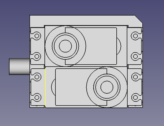
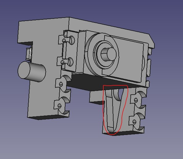
Assemble the Right and Left Sides:
- The entire right side should look like the image provided, and the left side should be a mirror image of the right.
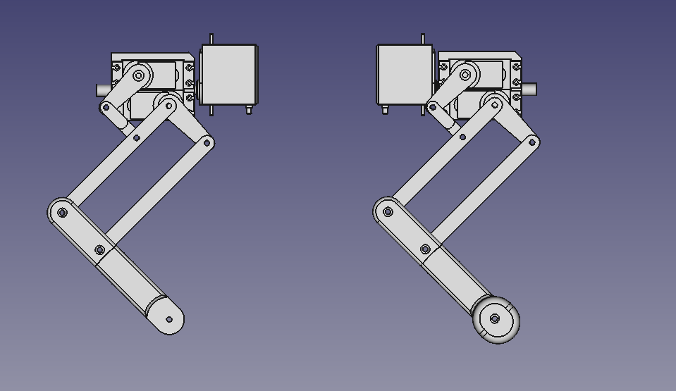
Mounting the Yaw Servos:
- Mount the servos that control the yaw of the leg. Ensure that the rotating part is on the bottom for all four servos.
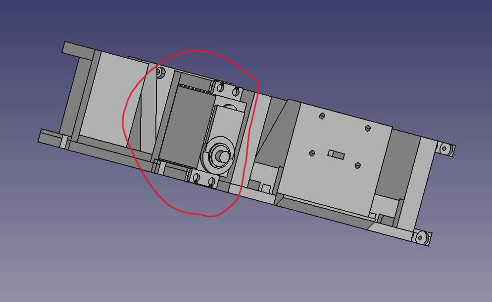
Final Assembly:
- Attach the servo horns to the shoulder servos in the body.
- Screw the front and back bumpers to the body.
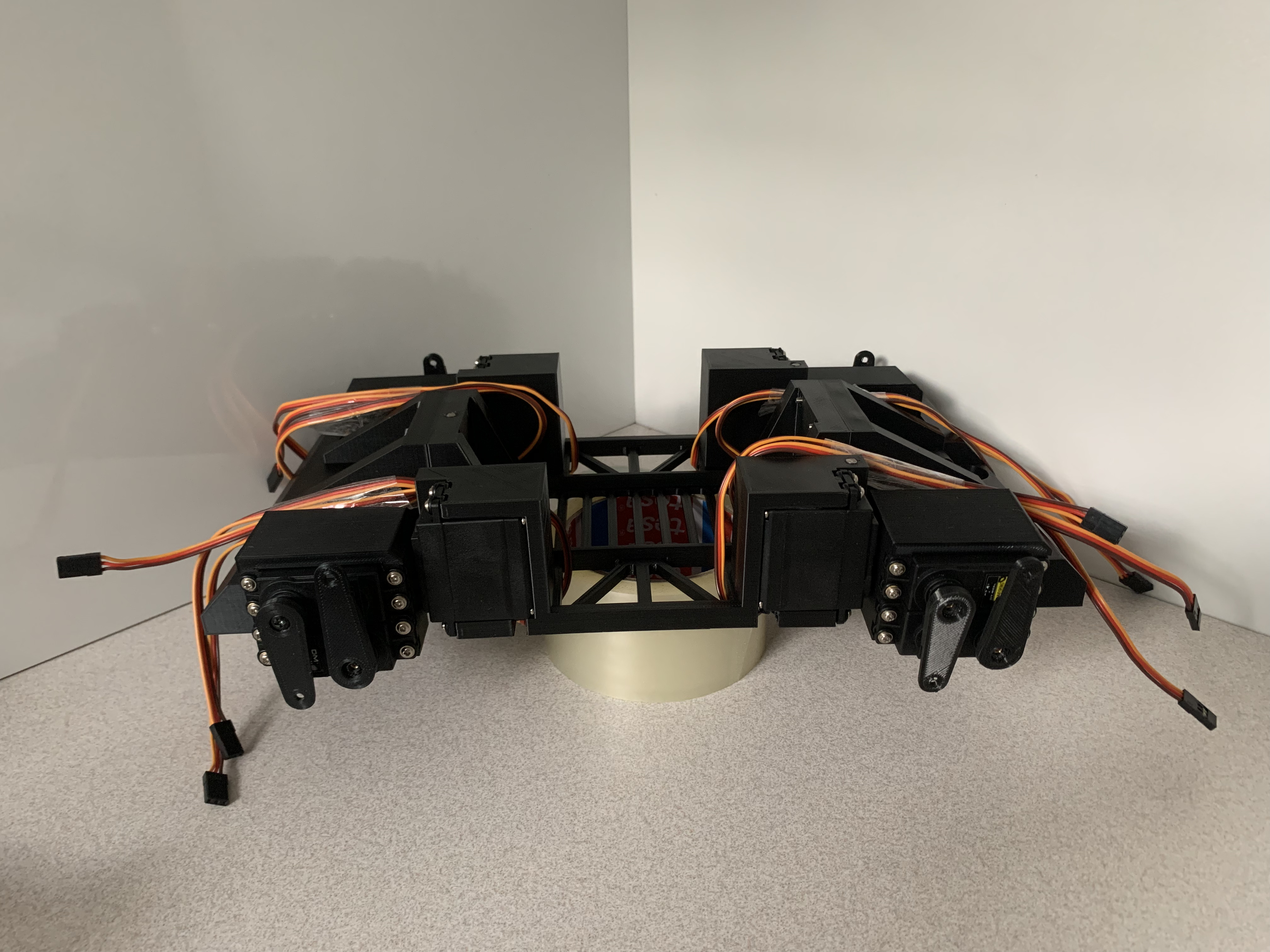
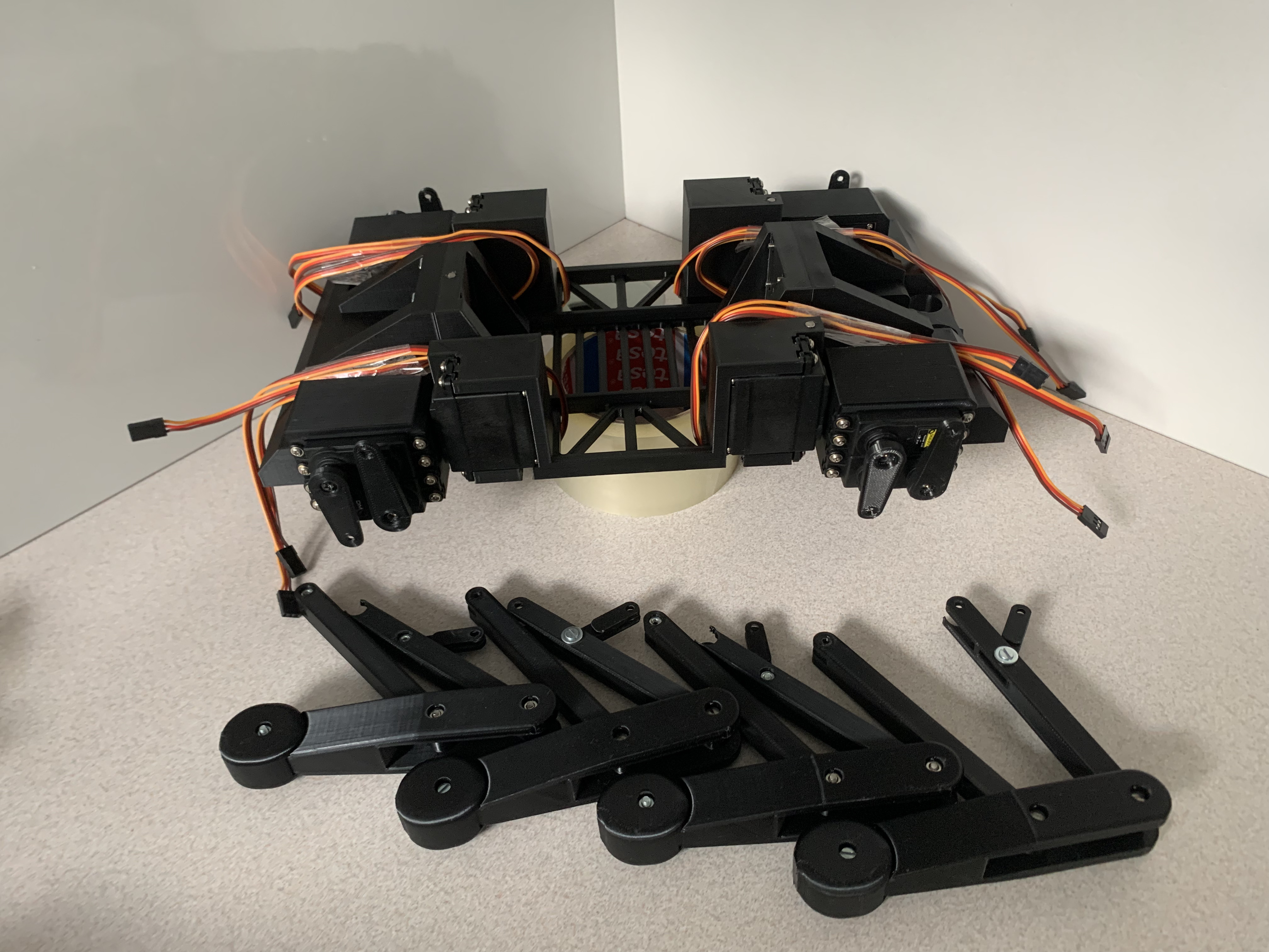
After completing these steps, you are now ready to move on to the next phase: hardware design.
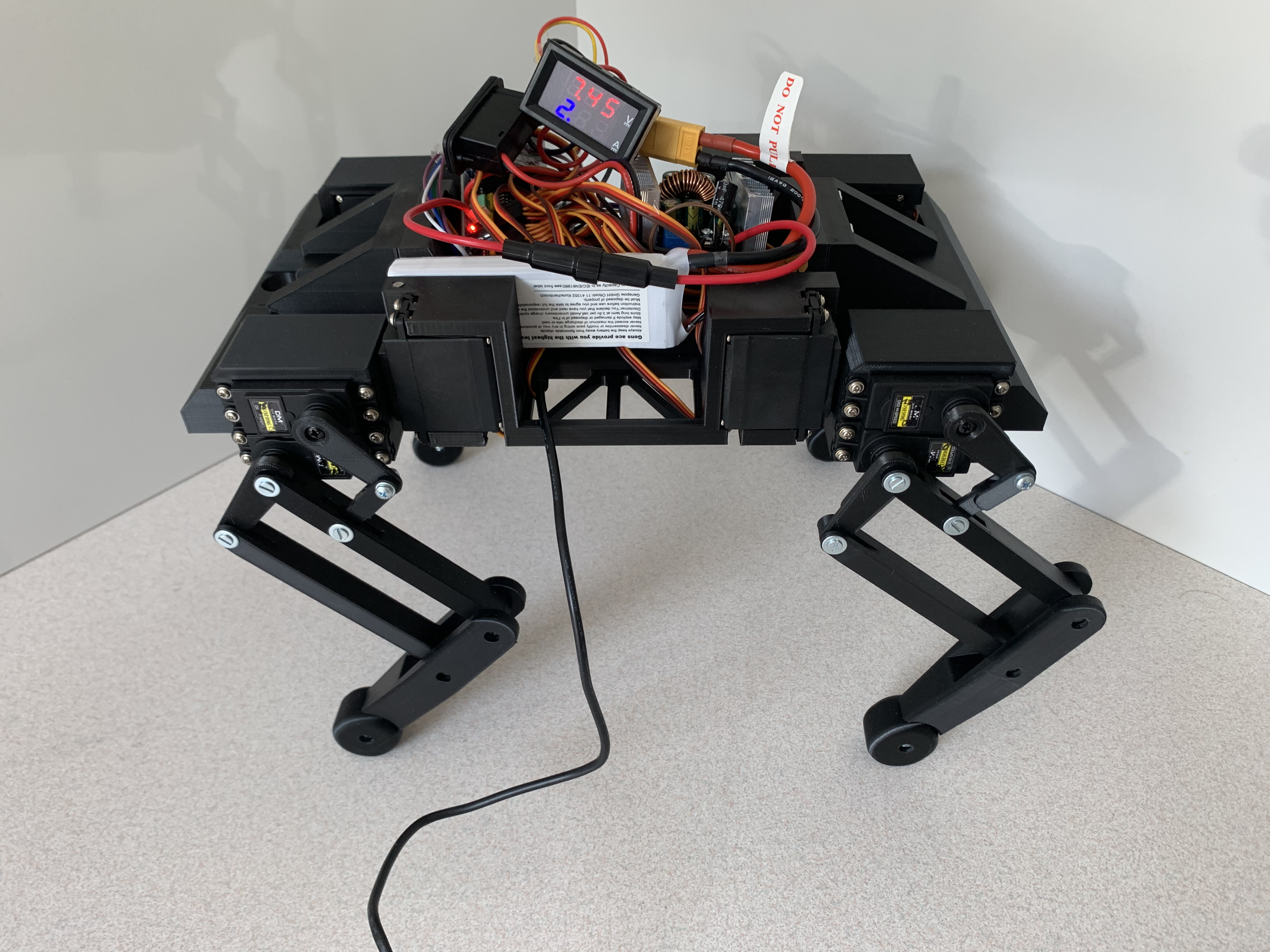
Hardware
Due to my limited knowledge of electronics, I aimed to keep things simple—unfortunately, this approach led to some significant mistakes. Below, I’ve provided a hardware diagram of my design, but I also want to share ways I could have improved it to help you avoid the same errors.

For many, it's obvious why we should use an external power supply for servos and a separate power source for the Raspberry Pi. However, for those less familiar with the reasoning, let me explain in more detail. Powering the PCA9685 module (which acts as a signal and power splitter for the servos) from the Raspberry Pi's 5V pin is not ideal. While the voltage might seem sufficient—since servos can operate between 4.8V and 6-7V—the real issue lies in the current draw.

My AC-DC power adapter(for Raspberry Pi) outputs 5.1V, which is almost directly supplied to the Raspberry Pi's 5V pin (with only a diode along the way, causing a minor 0.1V drop). So, when we draw current from the 5V pin, it comes directly from the adapter. My adapter supplies around 3.0A, which seems like a lot. However, we also need to consider the Raspberry Pi's current draw, which is about 700mA. That leaves us with roughly 2300mA (3000mA - 700mA), which still seems reasonable.
But here's the catch: if we calculate the current needed by the servos, 2300mA quickly becomes insufficient. According to the datasheet, a single servo can draw up to 1300mA while moving. Multiply that by 12 servos (assuming all are moving at once), and you get a total of 15,600mA. Now, that 2300mA seems insignificant. Even if only 8 servos are moving at once (such as during walking), the current draw still reaches 10,400mA—far more than what the power supply can handle.
In the worst-case scenario, if all the servos are blocked, they can draw up to 2500mA each, leading to a total of 30A (known as the stall current). Because of this, you need a robust battery that can handle such a high current draw (at least 30C) and a reliable buck converter to drop the voltage from 7.4V to 6V. However, finding a compact and affordable buck converter that can handle this isn't easy (which was one of my main project goals). As a compromise, I used a buck converter rated for 20A, with a fuse that will break if the current exceeds that limit.
My biggest mistake, however, was not splitting the 12 servos across 4 modules, one for each leg. If I had done this, I could have replaced the PCA9685—16-channel PWM servo controller—with 4 smaller controllers, each with 3 signal outputs. This would have reduced the risk of overloading the buck converter, servo controller, or even the Raspberry Pi in case of backflow current. With the servos split into modules, the highest possible current per module would be only 7.5A, with an average of around 2.5A—far more manageable than 10A! Moreover, a smaller and lighter buck converter would have increased the robot's possible payload.
Another issue I encountered was purchasing low-quality, cheap servos. Often, they would get stuck close before reaching the final position, which caused the stall current and, if left unchecked, could burn out the servos. They also had a tendency to skip steps. So, I learned a valuable lesson: cheap components may not always be the best option for projects like this.
Also small recommendation: when testing code, switch the power supply for the servos back to the Raspberry Pi's 5V pin and place the robot on a pedestal to minimize the load on the servos. The 2300mA should be enough for testing without damaging any parts. One thing I must admit: the torque of these servos is enormous!
Code
I won’t be uploading the entire code here, but I’ll explain the key concepts and the hidden math behind it. If you’d like to download the full code, you can find it on my GitHub. Additionally, I won’t cover the leg inverse kinematics, as I've already described in a previous post.
The core idea was to store the servo positions in a Python dictionary, allowing the foot’s position to be executed simultaneously. The process starts with calculating the angle for each servo based on the desired foot position. Once all the calculations are completed, they are stored in the dictionary. The next step is reading the data from the dictionary and writing it to the corresponding servo. This is where the write_servo function comes in—it reads the data from the dictionary and sends the appropriate commands to the servos.
Dictionary Abbreviations:
- FR - Front leg, Right side
- FL - Front leg, Left side
- BR - Back leg, Right side
- BL - Back leg, Left side
- S1 - Servo on the top
- S2 - Servo on the bottom
- S3 - Servo attached to the shoulder
Servo Offsets:
One important thing to consider is the offset for each servo. The 0-degree position for one servo might not correspond to the same position in the real world for another servo. For example, comparing FRS1 and FLS1, if we want them to form a mirror image, we need to apply the appropriate offset. As you may recall from the marks made during calibration, the 180-degree position for FLS1 is at the top, while for FRS1, it’s at the bottom.
To handle this, we’ll use basic trigonometry to adjust the system so that the 0-degree position is consistent across all servos. Imagine a semicircle with 180 degrees. Initially, we assume the 0-degree point is at the top, but we need it to be at the bottom. Using this adjustment ensures that the servos move in sync, maintaining proper alignment and motion.
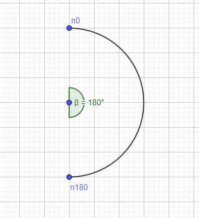
If we want to move our 0-degree point to the bottom of the semicircle (which is halfway around the semicircle), we need to shift the reference by 180 degrees, or π radians. To do this, we simply add π to our equation. This adjustment ensures that when we refer to 0 degrees, it will be positioned at the bottom, not the top.
By adding this π offset, our system correctly interprets the servo's position. So, for example, when the system calculates a 0-degree angle for a servo, it now knows that this position corresponds to the bottom of the semicircle, achieving the desired alignment and ensuring consistent movement across all servos.
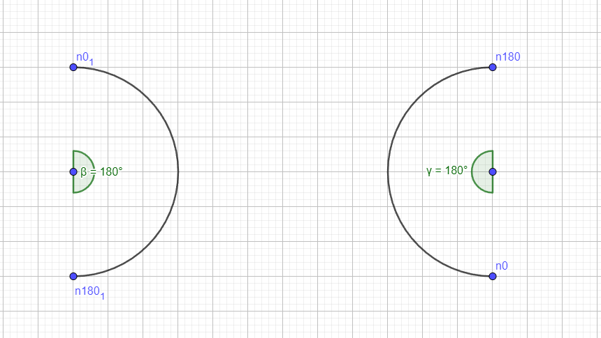
However, a new challenge arises: we want the range of movement on the right side, not on the left, as shown in the diagram. To achieve this, we need to modify our calculation. Instead of adding π to the equation, we will subtract the desired angle from π. This adjustment shifts the 0-degree position to the bottom while keeping the servo's range of movement on the right side.
Our new equation becomes:
\(\pi - desired_{point}\)
To convert this from radians to degrees, we multiply the result by \(\frac{180}{\pi}\). This formula allows us to create the correct offset for the servos, enabling the system to mirror the movements properly.
Example:
Let’s assume we want both the left and right servos to reach a position of 30 degrees (calculated from inverse kinematics). For the right servo, it's straightforward because the 0-degree point is already at the bottom. We simply add 30 degrees, and the servo reaches the correct position.
For the left servo, we apply the formula:
\(\pi - desired_{position} = \pi - 30 \frac{\pi}{180} = 150°\)
Now, we have a perfect mirror image of the right servo's position!
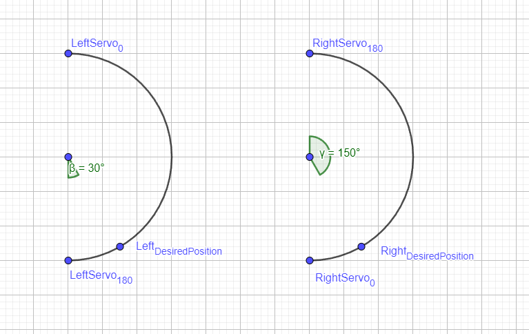
At the end of the process, we just need to determine the offset for each servo, so that the output of the inverse kinematics function will be identical on both sides of the robot.
This function is also a great place to make fine adjustments for each servo (in degrees) in case the assembly didn’t go perfectly, as was the case with mine. Since each setup might vary slightly, you’ll need to adjust the servos by setting the starting position and verifying if the legs are aligned with each other.
Starting position
The "starting_position" function is the initial phase to set a reference point. It uses the lists "starting_foot_cords_front" and "starting_foot_cords_back". The first value in each list represents the yaw of the leg in centimeters (reducing this value will move the foot inward toward the body). The second value indicates if the leg should be positioned more forward (positive) or backward (negative). The third value is the height. All values are given in centimeters, so if you input [0, 0, 15], the robot will be 15 cm tall, with the foot aligned with the rotating part of the bottom servo (S2).
Pitch
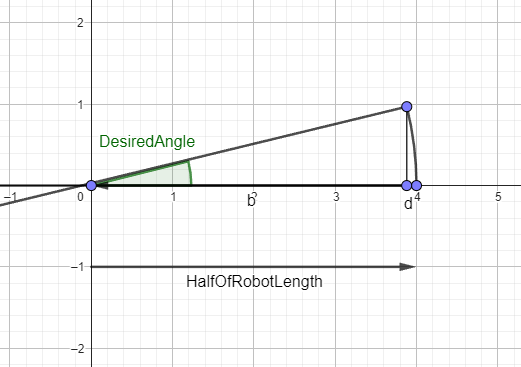
The next function is pitch, which controls how much the robot should tilt forward. If we know the robot’s length and the desired angle, we can calculate this movement. To make the concept easier to understand, refer to the diagram below. The formula is derived as follows:
-
From the equation \(\cos(\alpha) = \frac{b}{c/2}\), where \(b=\frac{c}{2}* \cos(\alpha)\), and \(b+d=\frac{c}{2}\), we get the formula for the change in d (the distance change after pitching):
\(d=\frac{c}{2}*(1-\cos(\alpha))\) -
We also need to calculate the height difference, so we can tilt the robot without changing the position of the feet. For the back legs, this would be:
\(z_B=h-\sin(\alpha)*\frac{robot_{length}}{2}\)And for the front legs:
\(z_F=h+\sin(\alpha)*\frac{robot_{length}}{2}\)
Now that we have the coordinates of the legs in the Cartesian coordinate system, we can input them into the "rad_to_degree" function to get the corresponding servo positions.
Walking mode
The last but certainly not least important function is the walking mode. This function is the most complex, as it uses a Bézier curve to create a smoother foot trajectory. I won’t dive too deeply into its mechanics here, as my understanding of the topic isn't advanced enough to explain the full mathematics behind it. However, I’ll briefly describe what it does. For more detailed information, I highly recommend reading the article "Leg Trajectory Planning for Quadruped Robots with High-Speed Trot Gait", which I referred to frequently throughout this project.
In essence, the Bézier formula helps create a smooth path between several points. Let’s say we provide three points: the starting point, the middle point, and the ending point. Using the Bézier formula, we can generate a smooth parabolic curve that allows the foot to move fluidly between these positions.
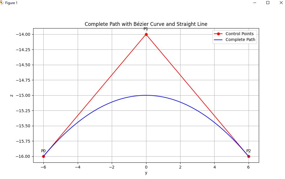
Using this formula and creating our path points we can get a very nice trajectory of the foot, based only on 12 points.
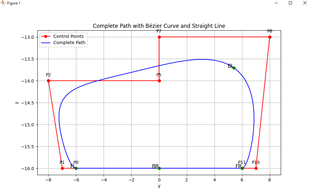
The movement of the foot can be divided into two phases: the stance phase and the swing phase. I decided to make the stance phase linear with a fixed speed, while the swing phase features acceleration and deceleration. Using the research from the previously mentioned report, we can introduce floating points to approximately control the speed of the leg at each point and manage the acceleration.
Once the foot's path is determined, the next step is coordinating the movement of all four legs. My goal was to mimic the walking cycle of a normal dog as closely as possible. After observing and studying the biology of a dog’s walk, I discovered that each leg's movement is delayed by 3/4 relative to the others. Since we have four legs, we can't split the movement evenly into four phases. Instead, each leg will always be in a different phase, but all legs will move in sync within the cycle.
Example:
At a given point in time:
- FR (Front Right) leg is in phase 1
- BR (Back Right) leg is in phase 2
- FL (Front Left) leg is in phase 3
- BL (Back Left) leg is in phase 4
The phases cycle in sync. After one cycle ends, FR moves to phase 2, BR to phase 3, FL to phase 4, and BL returns to phase 1. Each leg goes through all four phases over four cycles. The phases are represented by green points on the graph (shown above). For example:
- When FR is in phase 1, it moves from the ENDING point (P11) to the coordinate [0, height] (the MID point).
- Simultaneously, BR in phase 2 moves from the MID point to the STARTING point (P0).
- FL in phase 3 moves from the STARTING point to the 75% mark of the swing phase, known as the MOVE point.
- BL in phase 4 moves from the MOVE point to the ENDING point.
The phases are as follows:
- Phase 1: ENDING point → MID point
- Phase 2: MID point → STARTING point
- Phase 3: STARTING point → MOVE point
- Phase 4: MOVE point → ENDING point
This approach synchronizes the legs' movement while introducing a 3/4 phase delay between them.
Adjusting Walk Control Points:
You can modify the control points of the walking cycle as needed, but I recommend using small, fast steps to minimize balance issues. The prepare_to_walk and prepare_to_stop functions synchronize the transition between the starting position and walking, as well as from walking back to a stop.
The shift_list_right function manages the phases each leg is in. For example:
- First cycle:
['FR', 'BR', 'FL', 'BL'] = [phase1, phase2, phase3, phase4] - Next cycle:
['BL', 'FR', 'BR', 'FL'] = [phase1, phase2, phase3, phase4]
Finally, the cords_respect_CoM (Center of Mass) function is reserved for future development using a different coordinate system. Currently, we are using a single coordinate system—the tool coordinate system, which, for our purposes, could be better named the leg coordinate system.
If you want to see some videos of the performance, here is the link.
Conclusion
To summarize this project, there were definitely some mistakes and areas that could have been improved. However, it has been an incredibly valuable learning experience. There’s a good chance I’ll revisit this project in the future to fix those mistakes and, as promised in the previous article, add a tower to control the robot using gestures.
You can find the code and 3D models in the provided links. I encourage others to develop this project further and to ask questions, as it is open source. Additionally, I highly recommend reading my other articles to get a more comprehensive understanding of this project.
"Lastly, I dedicate this project to my dear friend, who inspired me to become a better person every day and gave me an enormous amount of inspiration. You will always remain in our hearts. Rest in peace."
Comments
Marta
- 13 November, 2024
Mega stronka bracie👌🤪
Leave a comment